5. Study design
The phenotype of interest will define the GWAS design. Some phenotypes are quantitative like body mass index or fasting blood glucose while others are qualitative, binary phenotypes (e.g., Case/Control studies). Each type requires special preparation of the input data, proper selection of the statistical tests and mindful interpretation of the final results. This tutorial is an example for a Case/Control study.
To start, the cases and controls must be selected based on the inclusion and exclusion criteria for the project. Accordingly, a subset of the genotypic and phenotypic data should be established. Then, the possible correlation of the phenotype of interest should assessed with the genetic principal components in the studied population. The possible covariates that might affect the phenotype of interest must also be identified, but that will be done during the assessment of heritability of the phenotype in the studied population.
5.1. Explore phenotypes
5.1.1. What is your phenotype of interest?
As explained earlier, the GRLS phenotypic data is organized in modular data tables. Many clinical conditions are organized in tables by the affectd tissue. For example, several cutaneous disorders are grouped in a table named "conditions_skin.csv". Let us define our target phenotype and its tissure to start our GWAS
# Define the target phenotype and the affacted tissue
target="atopy"
tissue="skin"

# Let us explore how the data table looks like
less phenotypes/conditions_${tissue}.csv
5.1.2. Identify affected cases until last year
Most of the input files are designed to have 2 rows for each new year of study. The 1st row records the new phenotypes diagnosed only in that study year while the 2nd row records all phenotypes diagnosed from baseline through that study year. The column to_date is encoded 0 for the former and 1 for the latter. More can be read about the design of each table in the Data Commons of Morris Animal Foundation. For this tutorial, we will identify the cases as the dogs that showed the phenotypes at any year of the study.
# Define and create the GWAS output folder
gwas="gwas_${target}" && mkdir -p "$gwas"

# Identify the 2nd row of the last year of study for each dog
cat phenotypes/conditions_${tissue}.csv | awk 'BEGIN{FS=","}\
    NR==1{print $0;next}{if ($5==1) {\
    if (!($1 in max_year) || $3 > max_year[$1]) {
        max_year[$1] = $3;
        line[$1] = $0;
    }}}END{for (id in line) {print line[id];}}' | tr ',' '\t' > "$gwas"/conditions_${tissue}_lastYear.tab
5.1.3. Count the of cases of each phenotype
# Get the number of columns in the header.
num_columns=$(head -n 1 "$gwas/conditions_${tissue}_lastYear.tab" | awk -F"\t" '{print NF}')

# Loop over each column from the third till the last and print the sum.
for ((i=7; i<=$num_columns; i++)); do
    awk -v col="$i" 'BEGIN{FS=OFS="\t"}NR==1{dis=$col;next}{sum+=$col} END {print dis,sum}' "$gwas"/conditions_${tissue}_lastYear.tab
done > "$gwas"/conditions_${tissue}.no_of_cases
5.2. Sample selection
5.2.1 Select "cases" of a target phenotype
Tcol=$(head -n 1 "$gwas/conditions_${tissue}_lastYear.tab" | awk -F"\t" -v pheno="$target" '{for (i=7; i<=NF; i++){if($i==pheno)print i}}')
awk -v Tcol="$Tcol" 'BEGIN{FS=OFS="\t"}NR==1{print;next}{if($Tcol=="1")print}' "$gwas"/conditions_${tissue}_lastYear.tab > "$gwas"/conditions_${target}_lastYear.tab

tail -n+2 "$gwas"/conditions_${target}_lastYear.tab | cut -f1 > "$gwas"/${target}_cases.ids
5.2.2 Check for co-existing conditions
for ((i=7; i<=$num_columns; i++)); do
    awk -v col="$i" 'BEGIN{FS=OFS="\t"}NR==1{dis=$col;next}{sum+=$col} END {if(sum)print dis,sum}' "$gwas"/conditions_${target}_lastYear.tab
done > "$gwas"/conditions_${target}_lastYear_coexist.tab
5.2.3. Identify individuals to be excluded from controls
grep 'allergic_reaction\|seasonal_allergy\|angioedema\|facial_edema\|.*_dermatitis\|r_o_atopy\|vaccine_reaction' "$gwas"/conditions_${tissue}.no_of_cases > "$gwas"/${target}.to_be_excluded.lst
while read offTarget;do
  offTcol=$(head -n 1 "$gwas"/conditions_${tissue}_lastYear.tab | awk -F"\t" -v pheno="$offTarget" '{for (i=7; i<=NF; i++){if($i==pheno)print i}}')
  awk -F"\t" -v Tcol="$Tcol" -v offTcol="$offTcol" 'NR>1{if($Tcol!="1" && $offTcol=="1")print $1}' "$gwas"/conditions_${tissue}_lastYear.tab
done < <(cut -f1 "$gwas"/${target}.to_be_excluded.lst) | sort | uniq > "$gwas"/${target}.to_be_excluded.ids
5.2.4. Remove the excluded samples from the genotyping dataset (include the oldies if not testing a phenotype with high mortality in young age)
cat "$gwas"/${target}.to_be_excluded.ids | grep -Fwf - AxiomGT1v2.filtered.fam > "$gwas"/${target}.to_be_excluded.samples
grep ^Oldies AxiomGT1v2.filtered.fam >> "$gwas"/${target}.to_be_excluded.samples

plink2 --bfile AxiomGT1v2.filtered --chr-set 38 no-xy --allow-extra-chr \
       --remove "$gwas"/${target}.to_be_excluded.samples --maf 0.01 \
       --make-bed --output-chr 'chrM' --out "$gwas"/AxiomGT1v2.filtered.${target}
5.2.5. Exclusion of 1st degree relatives
Again, the genotyping data will be used to assess sample-distances and thus identify sample duplications. 0.177 (the geometric mean of 0.25 and 0.125) will be used as cutoff for the KING kinship coefficients to identify 1st degree relatives.
# First, identify possible related dogs.
plink2 --bfile "$gwas"/AxiomGT1v2.filtered.${target} --chr-set 38 no-xy --allow-extra-chr \
       --king-cutoff 0.177 \
       --out "$gwas"/AxiomGT1v2.filtered.${target}.1st_degree_relatives

# Now, those relatives can be removed to avoid inflation of false associations in the GWAS.
plink2 --bfile "$gwas"/AxiomGT1v2.filtered.${target} --chr-set 38 no-xy --allow-extra-chr \
       --remove "$gwas"/AxiomGT1v2.filtered.${target}.1st_degree_relatives.king.cutoff.out.id \
       --make-bed --output-chr 'chrM' --out "$gwas"/AxiomGT1v2.filtered.${target}.noRelatives
5.3. Generate the phenotype file
awk 'FNR==NR{a[$1]=1;next}{if(!a[$2])print $1,$2,"1";else print $1,$2,"2";}' "$gwas"/${target}_cases.ids "$gwas"/AxiomGT1v2.filtered.${target}.noRelatives.fam > "$gwas"/${target}.pheno
cat "$gwas"/${target}.pheno | cut -d" " -f3 | sort | uniq -c
5.4. Linkage disequilibrium (LD) analysis
5.4.1 LD estimation
- --r2 reports squared inter-variant allele count correlations.
- --ld-window-r2 variant pairs with r2 values < 0.2 are filtered out by default. This option is used to adjust this threshold.
- Every pair of variants with at least 10 variants between them, or more than 1000 kilobases apart, is ignored. The first threshold can be changed with --ld-window, and the second threshold with --ld-window-kb.
plink --bfile "$gwas"/AxiomGT1v2.filtered.${target}.noRelatives --chr-set 38 no-xy --allow-extra-chr \
      --r2 --ld-window-r2 0 --ld-window-kb 10000 --ld-window 100 \
      --output-chr 'chrM' --out "$gwas"/AxiomGT1v2.filtered.${target}.noRelatives.stats
Generate a histogram of r2.
awk -v size=0.01 'BEGIN{OFS="\t";bmin=bmax=0}{ b=int($7/size); a[b]++; bmax=b>bmax?b:bmax; bmin=b<bmin?b:bmin } END { for(i=bmin;i<=bmax;++i) print i*size,(i+1)*size,a[i]/1 }' <(tail -n+2 "$gwas"/AxiomGT1v2.filtered.${target}.noRelatives.stats.ld) > "$gwas"/AxiomGT1v2.filtered.${target}.noRelatives.stats.ld.r2_histo ## 155780 sequential markers have complete linkage
Create an LD Decay Plot. The key step is the "aggregate" function that calculate the mean R2 of all pair of variants at the same distance
cat "$gwas"/AxiomGT1v2.filtered.${target}.noRelatives.stats.ld | awk '/NR==1/{print;next}{x=$5-$2;if(x<100000)print}' > "$gwas"/AxiomGT1v2.filtered.${target}.noRelatives.stats.ld2

Rscript -e 'args=(commandArgs(TRUE));require(ggplot2);'\
'ld_data <- read.table(paste(args[1],"/AxiomGT1v2.filtered.",args[2],".noRelatives.stats.ld2",sep=""), header = TRUE);'\
'ld_data$Distance <- abs(ld_data$BP_B - ld_data$BP_A);'\
'average_r2 <- aggregate(R2 ~ Distance, data = ld_data, mean);'\
'jpeg(file = paste(args[1],"/LD_Decay.",args[2],".jpg",sep=""));'\
'ggplot(average_r2, aes(x = Distance, y = R2)) + geom_line() + theme_minimal() + labs(x = "Distance (bp)", y = "r2");'\
'dev.off();' "$gwas" "${target}"
5.4.2 LD pruning
For this tutorial, we will prune pairwise SNPs with R2 > 0.8 (using windows of 100kb and step size of 1 SNP)
plink2 --bfile "$gwas"/AxiomGT1v2.filtered.${target}.noRelatives --chr-set 38 no-xy --allow-extra-chr \
       --indep-pairwise 100kb 0.8 \
       --output-chr 'chrM' --out "$gwas"/AxiomGT1v2.filtered.${target}.noRelatives.LD_lst ## 397962 of 578651 variants removed

plink2 --bfile "$gwas"/AxiomGT1v2.filtered.${target}.noRelatives --chr-set 38 no-xy --allow-extra-chr \
       --extract "$gwas"/AxiomGT1v2.filtered.${target}.noRelatives.LD_lst.prune.in \
       --make-bed --output-chr 'chrM' --out "$gwas"/AxiomGT1v2.filtered.${target}.noRelatives.LD_prune ## 180689 variants remaining
5.4.3 LD re-evaluation
plink --bfile "$gwas"/AxiomGT1v2.filtered.${target}.noRelatives.LD_prune --chr-set 38 no-xy --allow-extra-chr \
      --r2 --ld-window-r2 0 --ld-window-kb 10000 --ld-window 100 \
      --output-chr 'chrM' --out "$gwas"/AxiomGT1v2.filtered.${target}.noRelatives.LD_prune.stats


# New histogram.
awk -v size=0.01 'BEGIN{OFS="\t";bmin=bmax=0}{ b=int($7/size); a[b]++; bmax=b>bmax?b:bmax; bmin=b<bmin?b:bmin } END { for(i=bmin;i<=bmax;++i) print i*size,(i+1)*size,a[i]/1 }'  <(tail -n+2 "$gwas"/AxiomGT1v2.filtered.${target}.noRelatives.LD_prune.stats.ld) > "$gwas"/AxiomGT1v2.filtered.${target}.noRelatives.LD_prune.stats.ld.r2_histo

# Compare the change.
paste "$gwas"/AxiomGT1v2.filtered.${target}.noRelatives.stats.ld.r2_histo "$gwas"/AxiomGT1v2.filtered.${target}.noRelatives.LD_prune.stats.ld.r2_histo | less
How does the LD Decay Plot look?
cat "$gwas"/AxiomGT1v2.filtered.${target}.noRelatives.LD_prune.stats.ld | awk '/NR==1/{print;next}{x=$5-$2;if(x<100000)print}' > "$gwas"/AxiomGT1v2.filtered.${target}.noRelatives.LD_prune.stats.ld2

Rscript -e 'args=(commandArgs(TRUE));require(ggplot2);'\
'ld_data <- read.table(paste(args[1],"/AxiomGT1v2.filtered.",args[2],".noRelatives.LD_prune.stats.ld2",sep=""), header = TRUE);'\
'ld_data$Distance <- abs(ld_data$BP_B - ld_data$BP_A);'\
'average_r2 <- aggregate(R2 ~ Distance, data = ld_data, mean);'\
'jpeg(file = paste(args[1],"/LD_Decay_after_prune.",args[2],".jpg",sep=""));'\
'ggplot(average_r2, aes(x = Distance, y = R2)) + geom_line() + theme_minimal() + labs(x = "Distance (bp)", y = "r2");'\
'dev.off();' "$gwas" "${target}"
5.5. PCA to identify population admixture and to assess distribution of cases
5.5.1. Calculation of PCA
The --pca function in Plink2 extracts top principal components from the variance-standardized relationship matrix (i.e. genomic relationship matrix). LD pruning is adviced before PCA to reduce the risk of getting PCs based on just a few genomic regions. This behaviour tends to prevent deflation of statistical testing results later.
plink2 --bfile "$gwas"/AxiomGT1v2.filtered.${target}.noRelatives.LD_prune --chr-set 38 no-xy --allow-extra-chr \
       --autosome --pca \
       --output-chr 'chrM' --out "$gwas"/AxiomGT1v2.filtered.${target}.noRelatives.LD_prune.pca
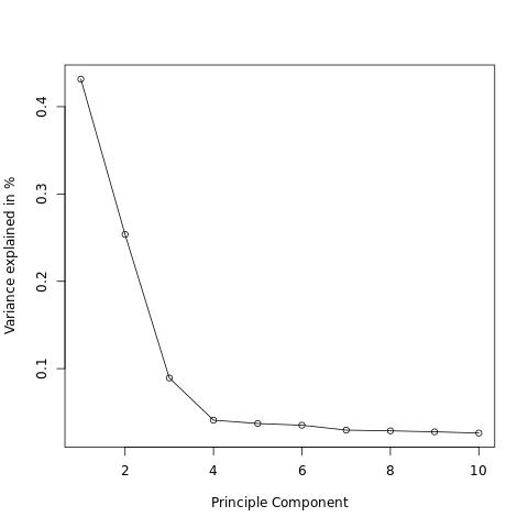
The variance can be plotted to identify the principal components that explain most of the variance.
Rscript -e 'args=(commandArgs(TRUE));'\
'val <- read.table(paste(args[1],"/AxiomGT1v2.filtered.",args[2],".noRelatives.LD_prune.pca.eigenval",sep=""));'\
'val$varPerc <- val$V1/sum(val$V1);'\
'jpeg(file = paste(args[1],"/Var_PCs.jpg",sep=""));'\
'plot( x = seq(1:length(val$varPerc)), y = val$varPerc, type = "o",xlab = "principal Component", ylab = "Variance explained in %");'\
'dev.off();' "$gwas" "${target}"
5.5.2. Assess possible batch effect
Plot the main principal components and color by the study batches:
Rscript -e 'args=(commandArgs(TRUE));require(ggplot2);require(gridExtra);'\
'eigenvec <- read.table(paste(args[1],"/AxiomGT1v2.filtered.",args[2],".noRelatives.LD_prune.pca.eigenvec",sep=""), header = TRUE, comment.char="");'\
'eigenvec$X.FID <-  as.factor(eigenvec$X.FID);'\
'plot1 <- ggplot(eigenvec, aes(x = PC1, y = PC2, col = X.FID)) + geom_point() + labs(title = "PCA Plot", x = "PC1", y = "PC2");'\
'plot2 <- ggplot(eigenvec, aes(x = PC3, y = PC4, col = X.FID)) + geom_point() + labs(title = "PCA Plot", x = "PC3", y = "PC4");'\
'plot3 <- ggplot(eigenvec, aes(x = PC1, y = PC3, col = X.FID)) + geom_point() + labs(title = "PCA Plot", x = "PC1", y = "PC3");'\
'plot4 <- ggplot(eigenvec, aes(x = PC2, y = PC3, col = X.FID)) + geom_point() + labs(title = "PCA Plot", x = "PC2", y = "PC3");'\
'combined_plot <- grid.arrange(plot1, plot2, plot3, plot4, nrow = 2);'\
'ggsave(paste(args[1],"/pca_plot.png",sep=""), combined_plot, width = 12, height = 8, dpi = 400);' "$gwas" "${target}"
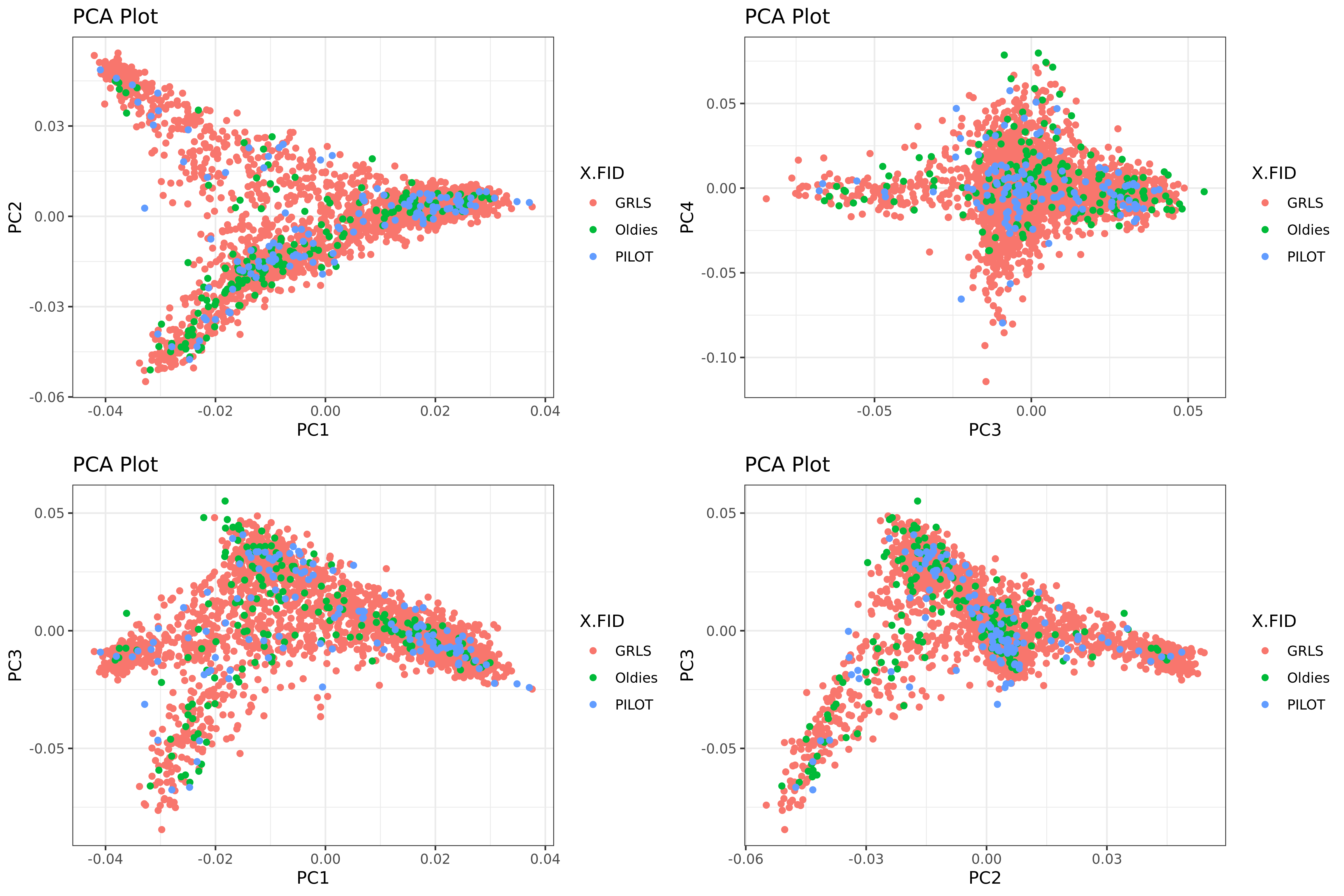
An additional tutorial of possible admixture analysis is here.
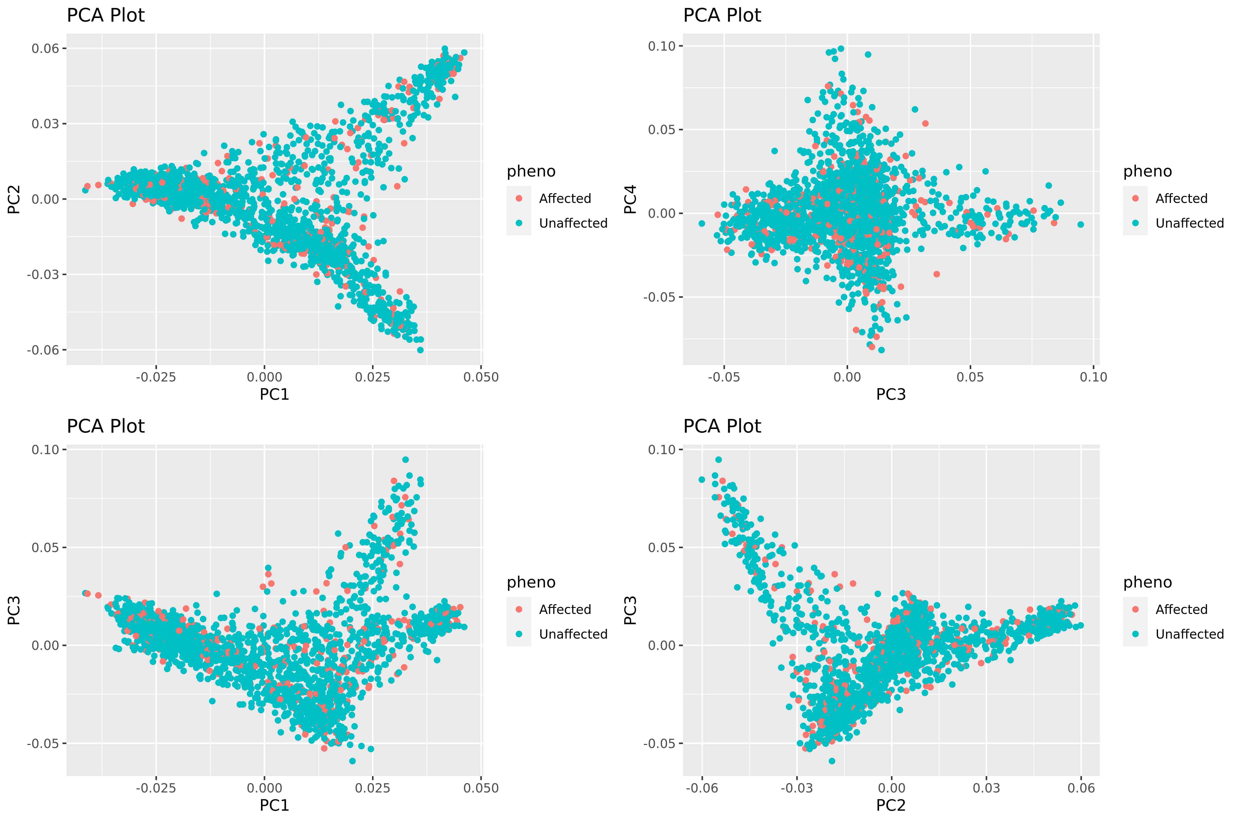
5.5.3 Assess distribution of cases in PCA
Rscript -e 'args=(commandArgs(TRUE));require(ggplot2);require(gridExtra);'\
'eigenvec <- read.table(paste(args[1],"/AxiomGT1v2.filtered.",args[2],".noRelatives.LD_prune.pca.eigenvec",sep=""), header = TRUE, comment.char="");'\
'pheno <- read.table(paste(args[1],"/",args[2],".pheno",sep=""), header = FALSE, comment.char="");'\
'names(pheno) <- c("FID", "IID", "pheno");'\
'pheno$pheno[pheno$pheno == "1"] <- "Unaffected";pheno$pheno[pheno$pheno == "2"] <- "Affected";'\
'ph_eigenvec <-  merge(pheno, eigenvec, by = "IID");'\
'ph_eigenvec$pheno <-  as.factor(ph_eigenvec$pheno);'\
'plot1 <- ggplot(ph_eigenvec, aes(x = PC1, y = PC2, col = pheno)) + geom_point() + labs(title = "PCA Plot", x = "PC1", y = "PC2");'\
'plot2 <- ggplot(ph_eigenvec, aes(x = PC3, y = PC4, col = pheno)) + geom_point() + labs(title = "PCA Plot", x = "PC3", y = "PC4");'\
'plot3 <- ggplot(ph_eigenvec, aes(x = PC1, y = PC3, col = pheno)) + geom_point() + labs(title = "PCA Plot", x = "PC1", y = "PC3");'\
'plot4 <- ggplot(ph_eigenvec, aes(x = PC2, y = PC3, col = pheno)) + geom_point() + labs(title = "PCA Plot", x = "PC2", y = "PC3");'\
'combined_plot <- grid.arrange(plot1, plot2, plot3, plot4, nrow = 2);'\
'ggsave(paste(args[1],"/pca_plot_",args[2],".png",sep=""), combined_plot, width = 12, height = 8, dpi = 400);' "$gwas" "${target}"